Starting with data frames

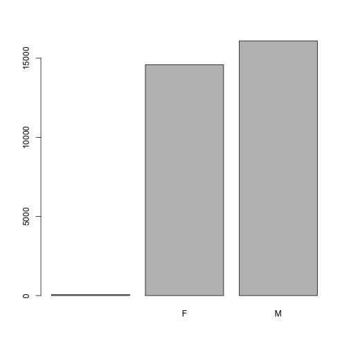
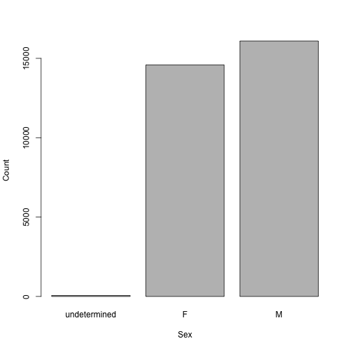
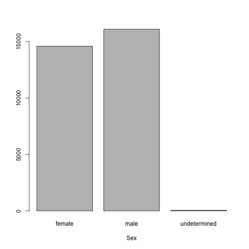
class: center, middle, inverse, title-slide

# Starting with data frames
## Data analysis and visualization in R <br> UC Merced
### Andrea Sánchez-Tapia <br> Rio de Janeiro Botanical Garden - ¡liibre! - RLadies+
### 2021-03-23

---

## last time

+ we setup a project and its file structure

+ we started using R inside RStudio

+ we created numerical, character and logical vectors with `c()`

+ we learned to subset vectors with brackets `[]` and other functions: `length()`, `:`, `seq(from, to, interval)`

+ vector subset can be done via numeric or logical indexes

---
## data structures in R

+ __vector__: lineal arrays (one dimension: only length)
--

+ __matrices__: arrays of vectors of the same type (all numeric or all character, for instance) (two dimensions: width and length)
--

+ __data frames__: two-dimensional structures ("rectangular") but might be of combined types (i.e., column 1 with names, column 2 with numbers)
--

+ __factors__: vectors (one-dimensional) representing __categorical variables__ and thus having __levels__
--

+ __lists__: literally lists, of objects that can be of any type (a list of data frames, or different objects)
--

+ __arrays__ are similar to matrices and dataframes but may be three-dimensional ("layered" data frames)

---
## matrices

+ data have to be of the same type

```r
?matrix
matrix(nrow = 4, ncol = 3)
```

```
##      [,1] [,2] [,3]
## [1,]   NA   NA   NA
## [2,]   NA   NA   NA
## [3,]   NA   NA   NA
## [4,]   NA   NA   NA
```

---
## matrices

+ you can also fit vectors with the correct dimensions

```r
nums <- 1:12
matrix(data = nums, nrow = 3)
matrix(data = nums, nrow = 3, byrow = TRUE)
```

---
## matrices

+ naming a matrix: `NULL or a list of length 2 giving the row and column names respectively.`  (?) look at the examples!

---
## matrices

```r
dim1_names <- c("row1", "row2", "row3")
dim2_names <- c("col1", "col2", "col3", "col4")
names_matrix <- list(dim_1 = dim1_names, dim_2 = dim2_names)
str(names_matrix)
m <- matrix(data = nums, nrow = 3,
       dimnames = names_matrix)
dim(m)
dimnames(m)
```
--

+ you can convert easily between data types `data.frame("m")`, `as.data.frame("m")`, `as.vector(m)`.
(the same goes for changes between "numeric", "logical")

---
class: inverse, middle, center
## starting with data frames

---
## the survey dataset

+ Data frames: one row per sampling unit (individual), one column per variable

---
## downloading the dataset

We are going to download the file to our `./data/raw` sub folder:

```r
download.file(url = "https://ndownloader.figshare.com/files/2292169",
              destfile = "./data/raw/portal_data_joined.csv")
```

---
## reading files into R

Functions to read data are key to any project.
for data frames: `read.csv()`, `read.delim()`

```r
surveys <- read.csv("./data/raw/portal_data_joined.csv")
surveys_check <- read.table(file = "./data/raw/portal_data_joined.csv",
                            sep = ",",
                            header = TRUE)
identical(surveys, surveys_check)
```

```
## [1] TRUE
```

---
## reading files into R

+ Package __readr__ 
+ Package __data.table__ (`data.table::fread()`) when you need to open a large file
+ Excel spreadsheets: `readxl::read_excel()`
+ __Graphic interface__

There are __many other ways__ to read data into R, some are specific for the type of data (GIS shapefiles or raster, and specific packages may come with their own reader functions)

---
## inspecting `data.frame` objects

```r
str(surveys)
dim(surveys)
nrow(surveys)
ncol(surveys)
head(surveys) # 6 rows by default
tail(surveys)
names(surveys)
rownames(surveys)
length(surveys) # number of columns
summary(surveys)
```

---
## inspecting `data.frame` objects

Based on the output of `str(surveys)`, can you answer the following questions?

+ What is the class of the object surveys?

+ How many rows and how many columns are in this object?

+ What is the type of data of the columns?

---
## indexing and subsetting data frames

+ a vector has only one dimension, so:

+ `length()` refers to number of __elements__
  + `dim()`
  + selection between brackets `[]`

+ a data.frame has __two__ dimensions: `dim()`, `ncol()`, `nrow()` selection between brackets `[]` __BUT with the two dimensions separated by a comma__: `[rows, columns]`

+ we'll try to refer to these operations as __selecting columns__ and __filtering rows__

---
## selecting columns

+ with numeric indexes and vectors

```r
surveys[, 6]
surveys[1, ]
surveys[ , 13]
surveys[4, 13]
surveys[1:4, 1:3]
```

---
## indexing and subsetting data frames

+ minus sign to __remove__ the indexed column or row

```r
# The whole data frame, except the first column
surveys[, -1]
nrow(surveys)
surveys[-(7:34786), ] # Equivalent to head(surveys)
```

---
## selecting columns by name

```r
names(surveys)

surveys["species_id"]       # Result is a data.frame
  surveys[["species_id"]]     # Result is a vector
* surveys[, "species_id"]     # Result is a vector
* surveys$species_id          # Result is a vector
```

+ R has several ways to do some things

---
## indexing and subsetting data frames

<small>

```r
sub <- surveys[1:10,]
# first element in the first column of the data frame

# first element in the 6th column

# first column of the data frame (as a vector)

# first column of the data frame (as a dataframe)

# first three elements in the 7th column (as a vector)

# the 3rd row of the data frame

# equivalent to head_surveys <- head(surveys)
```

---
## indexing and subsetting data frames

<small>

```r
sub <- surveys[1:10,]
# first element in the first column of the data frame
sub[1, 1]
# first element in the 6th column
sub[1, 6]
# first column of the data frame (as a vector)
sub[, 1]
# first column of the data frame (as a dataframe)
sub[1]
# first three elements in the 7th column (as a vector)
sub[1:3, 7]
# the 3rd row of the data frame
sub[3, ]
# equivalent to head_surveys <- head(surveys)
head_surveys <- surveys[1:6, ]
```

---
## challenge

<small>

+ Create a data.frame (`surveys_200`) containing only the data in row 200 of the `surveys` dataset

+ Notice how `nrow()` gave you the number of rows in a data.frame? Use that number to pull out just that last row in the data frame

+ Compare that with what you see as the last row using `tail()` to make sure it’s meeting expectations

+ Pull out that last row using `nrow()` instead of the row number.

+ Create a new data frame (`surveys_last`) from that last row.

+ Use `nrow()` to extract the row that is in the middle of the data frame. Store the content of this row in an object named `surveys_middle`.

+ Combine `nrow()` with the - notation above to reproduce the behavior of `head(surveys)`, keeping just the first through 6th rows of the surveys dataset.

</small>

---
## dealing with missing data

```r
sub <- surveys[1:10,]
#str(sub)
sub$hindfoot_length 
sub$hindfoot_length == NA #it cannot compare! because it's NA 
#we use is.na: 
#is.na(sub$hindfoot_length) # yes! returns a logical vector 
sub$hindfoot[!is.na(sub$hindfoot_length)]
```

---
## dealing with missing data

+ in some functions: `na.rm`

```r
mean(sub$hindfoot_length)
```

```
## [1] NA
```

```r
mean(sub$hindfoot_length, na.rm = T)
```

```
## [1] 31.5
```

---
## dealing with missing data

+ Dealing with missing data in dataframes: __filtering rows that have NAs__

```r
non_NA_w <- surveys[!is.na(surveys$weight),]
dim(non_NA_w)
```

```
## [1] 32283    13
```

```r
non_NA <- surveys[!is.na(surveys$weight) &
                    !is.na(surveys$hindfoot_length),]
dim(non_NA)
```

```
## [1] 30738    13
```

---
## dealing with NAs

```r
#complete.cases(surveys)
surveys1 <- surveys[complete.cases(surveys) , ]
surveys2 <- na.omit(surveys)
dim(surveys1)
```

```
## [1] 30738    13
```

```r
dim(surveys2)
```

```
## [1] 30738    13
```

---
## write csv objects to disk

```r
if (!dir.exists("data/processed")) dir.create("data/processed", recursive = T)
write.csv(surveys1, "data/processed/surveys_mod.csv")
```

#### remember you never overwrite your original, raw data!

---
## read the modified csv

```r
surveys <- read.csv("data/processed/surveys_mod.csv")
str(surveys)
```

---
## factors

+ __factors__: vectors (one-dimensional) representing __categorical variables__ and thus having __levels__. ordered (`c(“low”, “medium”, “high”)` or unordered (`c("green", "blue", "red")`)

+ R < 4.0 had a default behavior `stringsAsFactors = TRUE` so any character column was transformed into a factor

```r
`?read.csv()`
?default.stringsAsFactors
```

#### today if we want factors we have to transform the vectors

---
## factors

<small>

```r
## Compare the difference between our data read as
#`factor` vs `character`.
surveys <- read.csv("data/raw/portal_data_joined.csv",
                    stringsAsFactors = FALSE)
str(surveys)

surveys <- read.csv("data/raw/portal_data_joined.csv",
                    stringsAsFactors = TRUE)
str(surveys)
```

---
## factors

Convert the column "plot_type" and "sex" into a factor:

```r
surveys$plot_type <- factor(surveys$plot_type)
surveys$sex <- factor(surveys$sex)
```

(actually this is a way to create new columns)

---
## working with factors

<small>

```r
sex <- factor(c("male", "female", "female", "male"))
levels(sex) # in alphabetical order!
nlevels(sex)
sex
sex <- factor(sex, levels = c("male", "female"))
sex # after re-ordering
as.character(sex)
```

---
## let's make a plot of a factor variable

`plot(as.factor(surveys$sex))`

.pull-right[let's rename this label]

![](02_Starting_with_data_files/figure-html/plot-1.png)

---
## let's make a plot of a factor variable

`plot(sex)`

.pull-right[let's rename this label]

![](02_Starting_with_data_files/figure-html/plot2-1.png)

---
## challenge

<small>

.pull-left[
![](02_Starting_with_data_files/figure-html/remedy003-1.png)
]

.pull-right[

+ Rename “F” and “M” to “female” and “male” respectively.

+ Now that we have renamed the factor level to “undetermined”, can you recreate the barplot such that “undetermined” is last (after “male”)?
]

---
## some basic plotting

```r
plot(surveys$hindfoot_length)
plot(surveys$weight)
plot(sort(surveys$hindfoot_length))
plot(sort(surveys$weight))
```

---
## scatterplots

+ two continuous variables

```r
x <- surveys$weight
y <- surveys$hindfoot_length
plot(x, y) 
#but you can also avoid creating the vectors
plot(surveys$weight, surveys$hindfoot_length) #check the help for parameter order, x, y axis.
```

---
## boxplots

```r
head(surveys$plot_type)
levels(surveys$plot_type)
```

# boxplots

```r
plot(surveys$weight ~ surveys$plot_type)
```

+ check the __tilde__ `~` notation, formula:
"as a function of"

`plot(a ~ b)`
`plot(b, a)`

---
## plotting basics

all parameters for plotting are in function `par()`

```r
plot(x, y)
plot(x, y, xlab = "Hindfoot length", ylab = "Weight", cex = 0.9, pch = 19)
plot(x, y, xlab = "Hindfoot length", ylab = "Weight", cex = 0.9, pch = 19, col = "red")
plot(x, y, xlab = "Hindfoot length", ylab = "Weight", cex = 0.9, pch = 19, col = surveys$sex)
```

+ pch, cex, xlab, ylab,

+ __saving a plot!__

---
class: center, middle
# ¡Thanks!

<center>
<svg viewBox="0 0 512 512" style="position:relative;display:inline-block;top:.1em;fill:#A70000;height:1em;" xmlns="http://www.w3.org/2000/svg">  <path d="M476 3.2L12.5 270.6c-18.1 10.4-15.8 35.6 2.2 43.2L121 358.4l287.3-253.2c5.5-4.9 13.3 2.6 8.6 8.3L176 407v80.5c0 23.6 28.5 32.9 42.5 15.8L282 426l124.6 52.2c14.2 6 30.4-2.9 33-18.2l72-432C515 7.8 493.3-6.8 476 3.2z"></path></svg> [andreasancheztapia@gmail.com](mailto:andreasancheztapia@gmail.com)